PSA User Guide
PSA-Server can be used for computing physico-chemical properties of protein from the sequences.
The server can take either
(1) A group/ensemble of protein sequences (ESEQ), or
(2) Multiple Sequence Alignment data (MSA), as input.
In both the cases, sequences have to be in FASTA format. Both the options are described below along with the outputs.
Sample outputs for both the cases can be accessed from : ESEQ and MSA
1. Ensemble of protein sequences in FASTA format
Input preparation and job submission
PSA works on protein sequences with one-letter codes for amino acids.
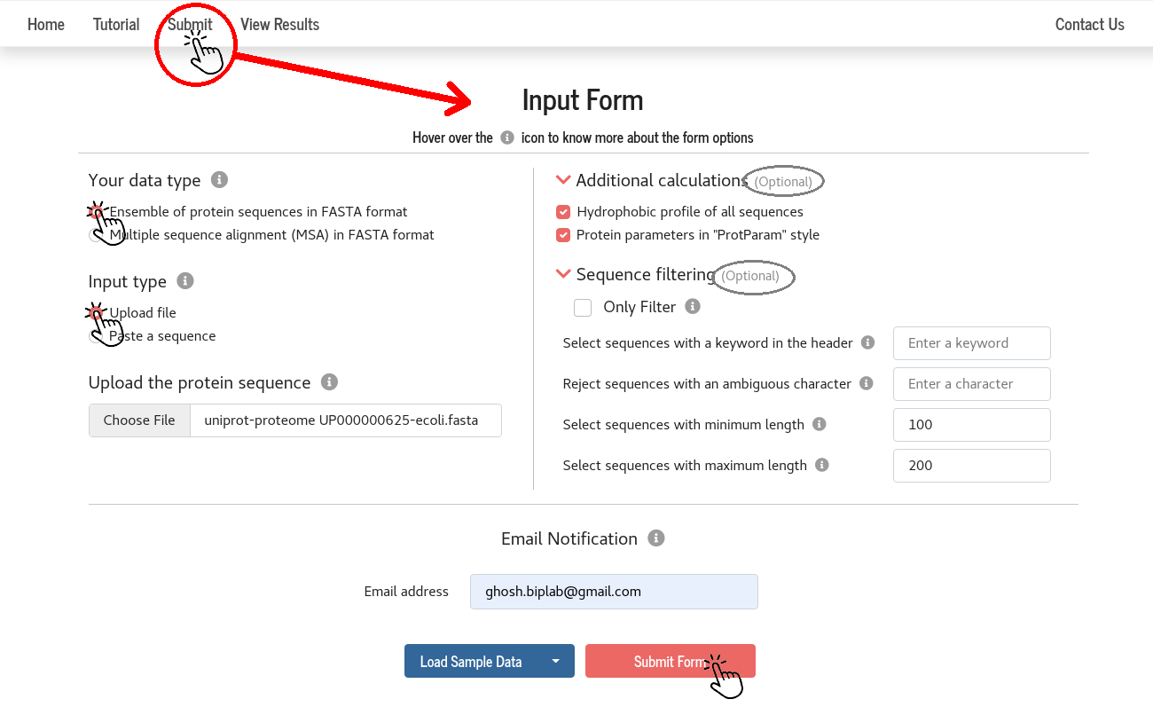
Users can either upload a file (file name must have the extension “.fasta”) containing all the sequences or paste the sequences in the given box.
The sequences can be separated by at least one blank line or the header line starting with the character “>”.
Following are some correct ways of preparing the input:
> Sequence-1
EFGHIYKFKDCSKVITGLHPTQAPTHLSVDTKFKTEGLCVDIPKDMT
> Sequence-2
AENVTGLFKDCSRVITGLHPTQAPTALSVDTKFKTEGLCVDIPGIPKDMT
> Sequence-3
MENEFIYKLMNPQRITGLHPTQAPTCLSV DTKFKTEGLCVDIPGIPKDMT
> Sequence-1
EFGHIYKFKDCSKVITGLHPTQAPTHLSVDTKFKTEGLCVDIPKDMT
> Sequence-2
AENVTGLFKDCSRVITGLHPTQAPTALSVDTKFKTEGLCVDIPGIPKDMT
> Sequence-3
MENEFIYKLMNPQRITGLHPTQAPTCLSV DTKFKTEGLCVDIPGIPKDMT
EFGHIYKFKDCSKVITGLHPTQAPTHLSVDTKFKTEGLCVDIPKDMT
AENVTGLFKDCSRVITGLHPTQAPTALSVDTKFKTEGLCVDIPGIPKDMT
MENEFIYKLMNPQRITGLHPTQAPTCLSV DTKFKTEGLCVDIPGIPKDMT
Inputs in the right column of the “Input form” are optional.
By choosing the suitable “filtering options”, one can select sequences for analysis using PSA.
The duly filled “Input Form” can be submitted to the server by clicking the “Submit Form” button.
Users may provide their email (optional) to receive a “Job completion” notification.
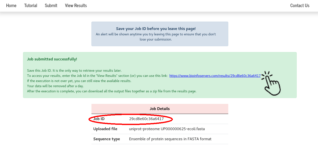
A “Job ID” and the link to view the results are provided on submission. By clicking the link, one can directly go to the results page.
One can also navigate to the results page by entering their “Job ID” in the View Results section.

Viewing the results
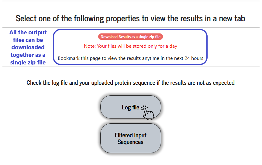
Available results are displayed in a grid of coloured boxes, and a result can be viewed by clicking on the relevant “coloured box” in the grid. The result files (raw data files) are stored for 24 hours and can be downloaded as a single zip file.


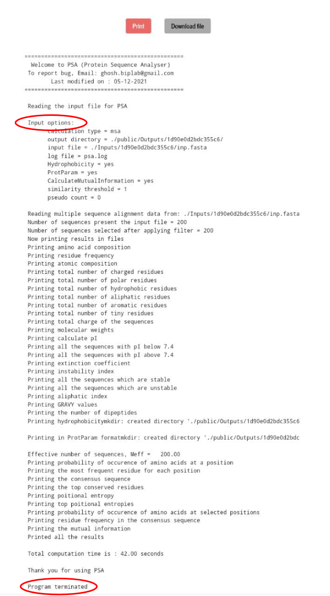
Errors and PSA execution progress are logged in this file. On completion of execution, “Program terminated” is printed at the end. Users are advised to see this log file and analyse the errors (if any).


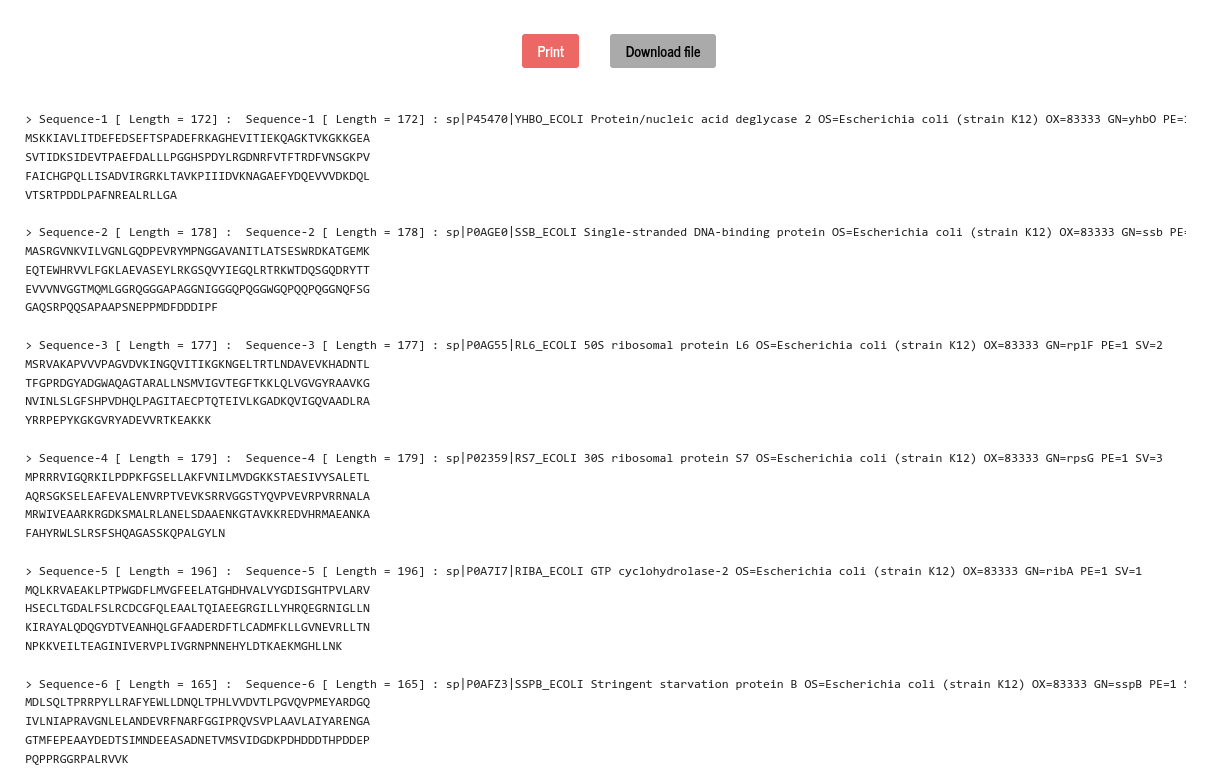
Sequences used in the PSA calculations are listed here. Each sequence is numbered and referred to as “Sequence number”. The ensemble of sequences can be downloaded as a file.


Aliphatic index of a protein is deducible from its sequence, and it is defined as the relative volume of a protein occupied by the aliphatic side chains (Alanine, Valine, Isoleucine, and Leucine). Aliphatic index has been found to have a positive correlation with the thermostability of proteins. Aliphatic index is calculated using the following formula (J. Biochem. 88, 1895-1898, (1980)):
\(Aliphatic~~index = x_A + a\times x_V + b\times (x_I+x_L)\)
Where \(a=2.9\) and \(b=3.9\); \(~x\) represents the mole percent (\(100~\times\) mol fraction) of the amino acid in the subscript.
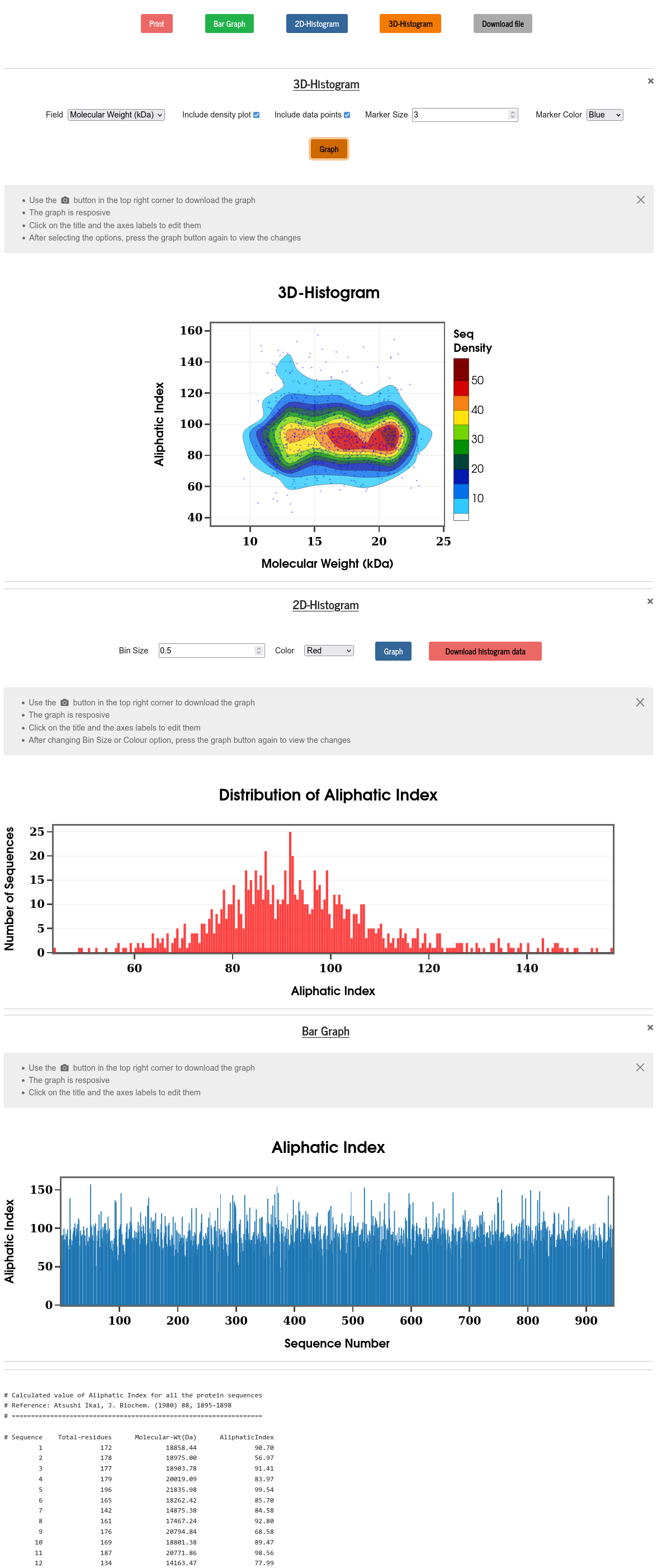
PSA calculates the aliphatic index of all the given sequences and displays them against the sequence number in a bar graph, or in the form of 2D and 3D histograms. The raw numerical data is also displayed and can be downloaded. Users are given various control to modify plots.

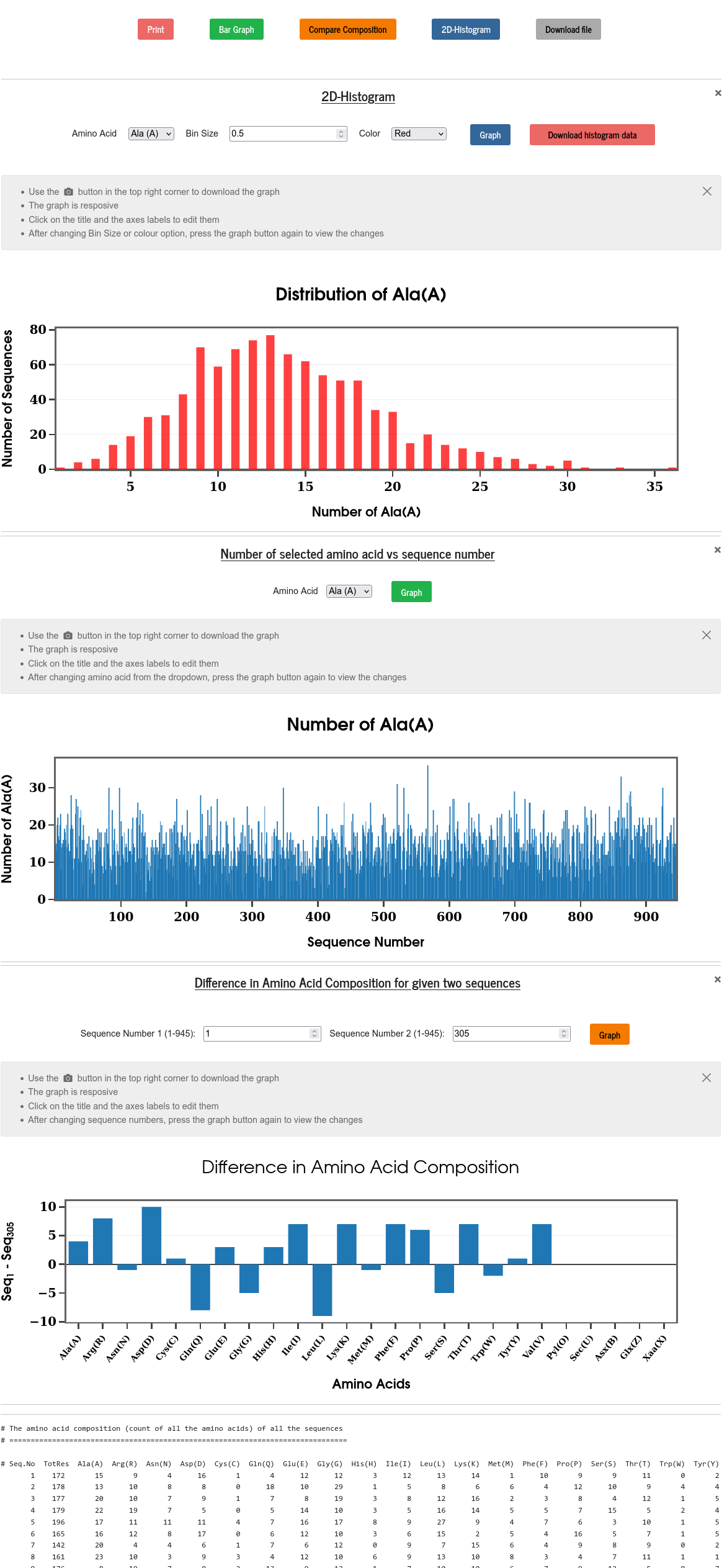
The amino acid composition of a protein sequence is obtained by counting the occurrence of each of the amino acids in the sequence. The amino acid composition is also normalized by the total number of residues (i.e., the sequence length) and made available to the user on a separate result tab. The results can be viewed in the form of the number or fraction of each amino acid in all the sequences, also as the distribution (2D histogram) of each of the amino acids across the whole set of sequences. Users can also compare the composition of two given sequences. Users are given control to choose bin size, labels of the plots, and also the range of the axes.

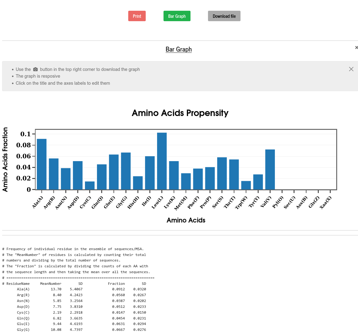
The propensity of an amino acid is calculated from the set of sequences as the ratio of the total number of that amino acid to the total number of amino acids of all types. Along with the raw data, the propensity is shown as a bar diagram for all the amino acids.
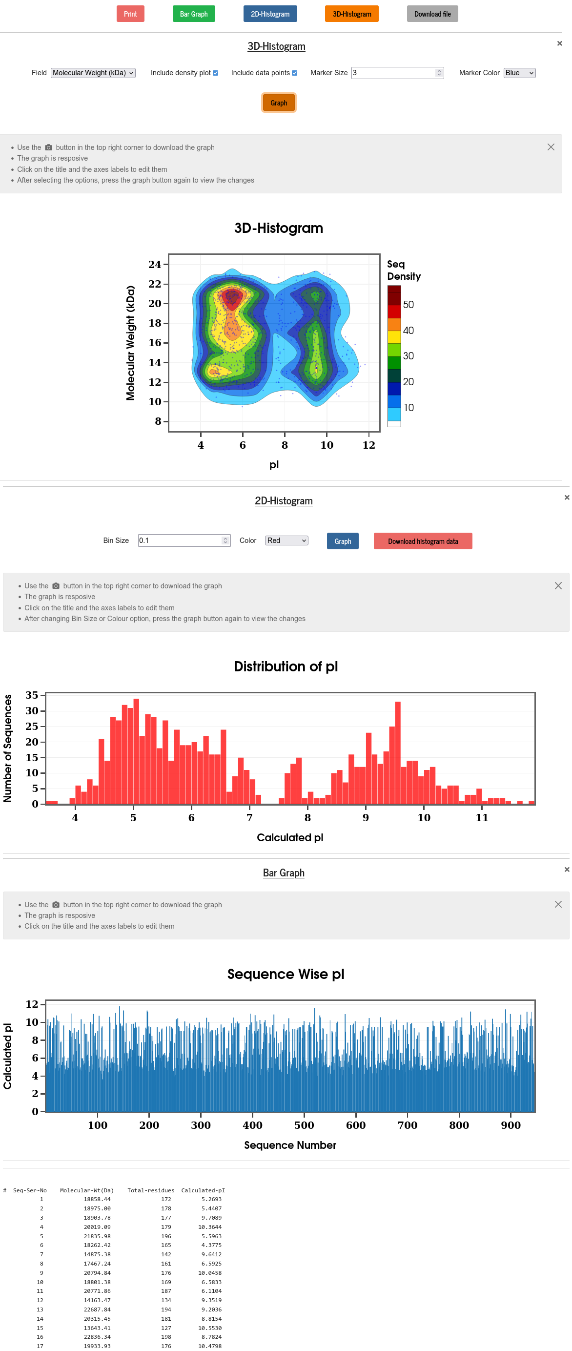
Isoelectric point (pI) refers to the pH at which a particular molecule carries no net electrical charges. For proteins, pI is a critical parameter for various biochemistry and proteomics techniques (e.g., 2D gel electrophoresis (2D-PAGE)). Here, pI is calculated using pK values of amino acids as described in Bjellqvist et al. (Electrophoresis, 15, 529-539, 1994) and displayed against the serial numbers of the selected sequences and in the form of a frequency distribution (histogram). The raw data is also displayed and can be downloaded from the “Download file” button. The algorithm used in PSA does not account for the effects of post-translational modifications.

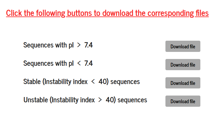
Input sequences are clustered into four categories based on the calculated values of pI and the instability index. The files can be downloaded from their respective “Download file” link. The downloaded sequence files can be used as input for a new PSA calculation.

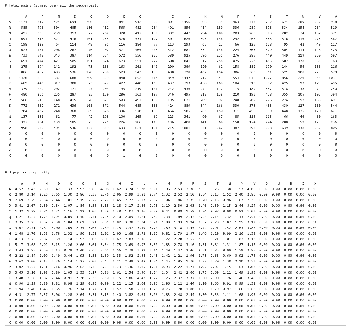
The propensity of amino acid pairs in a sequence can be calculated from the composition of dipeptides in the sequence. Counts of occurrence of all the possible pairs of residues (dipeptides) are displayed in the form of a matrix for each sequence. At the end of this file, a total number of pairs (summed over all the sequences) and the propensity of a pair of residues (dipeptide propensity) are also displayed and shown in the figure. Dipeptide propensity for a pair of residues \(x,y\) is calculated using the following formula:
\(propensity(x,y) = 100 \times \frac{\sum\limits_{i}N^{i}_{xy}}{\sum\limits_{i}^{ }N^{i}_{x} + \sum\limits_{i}^{ }N^{i}_{y}}\)
Where the summation is over all the sequences; \(~N^{i}_{xy}~\) is the number of dipeptides \(~xy~\) in the \(~i^{th}~\) sequence and \(~N^{i}_{x}~\) is the number of \(~x~\) residue in the \(~i^{th}~\) sequence.

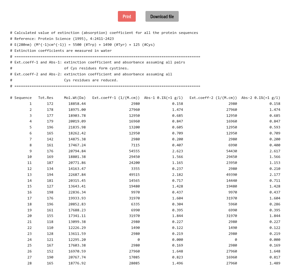
The extinction coefficient is a measure of absorption of light of a certain wavelength in a protein solution and is used to determine the concentration of protein in UV spectrometry. The molar extinction coefficient can be estimated (Analytical Biochemistry, 182, 319-326(1989)) from the composition of amino acids in a protein sequence. For a denatured protein, the molar extinction coefficient (at 280 nm) can be computed from the number of Tryptophan, Tyrosine and Cysteine residues in the molecule and using the following formula (Protein Science, 4:2411-2423, (1995)):
\( \epsilon_{280}(M^{-1} cm^{-1}) = 5500\times n_{Trp} + 1490\times n_{Tyr} + 125\times n_{cystine}\)
Where \(~n~\) is the number of amino acid in the subscript. As cysteine does not absorb appreciably at wavelengths > 260 nm, but cystine does, the extinction coefficient is printed in two different columns in the table corresponding to the two cases. The absorbance (optical density) is calculated as \(~\frac{\epsilon_{280}}{MWt}~\). The extinction coefficient and the absorbance of all the protein sequences are calculated, and presented in a tabular format.

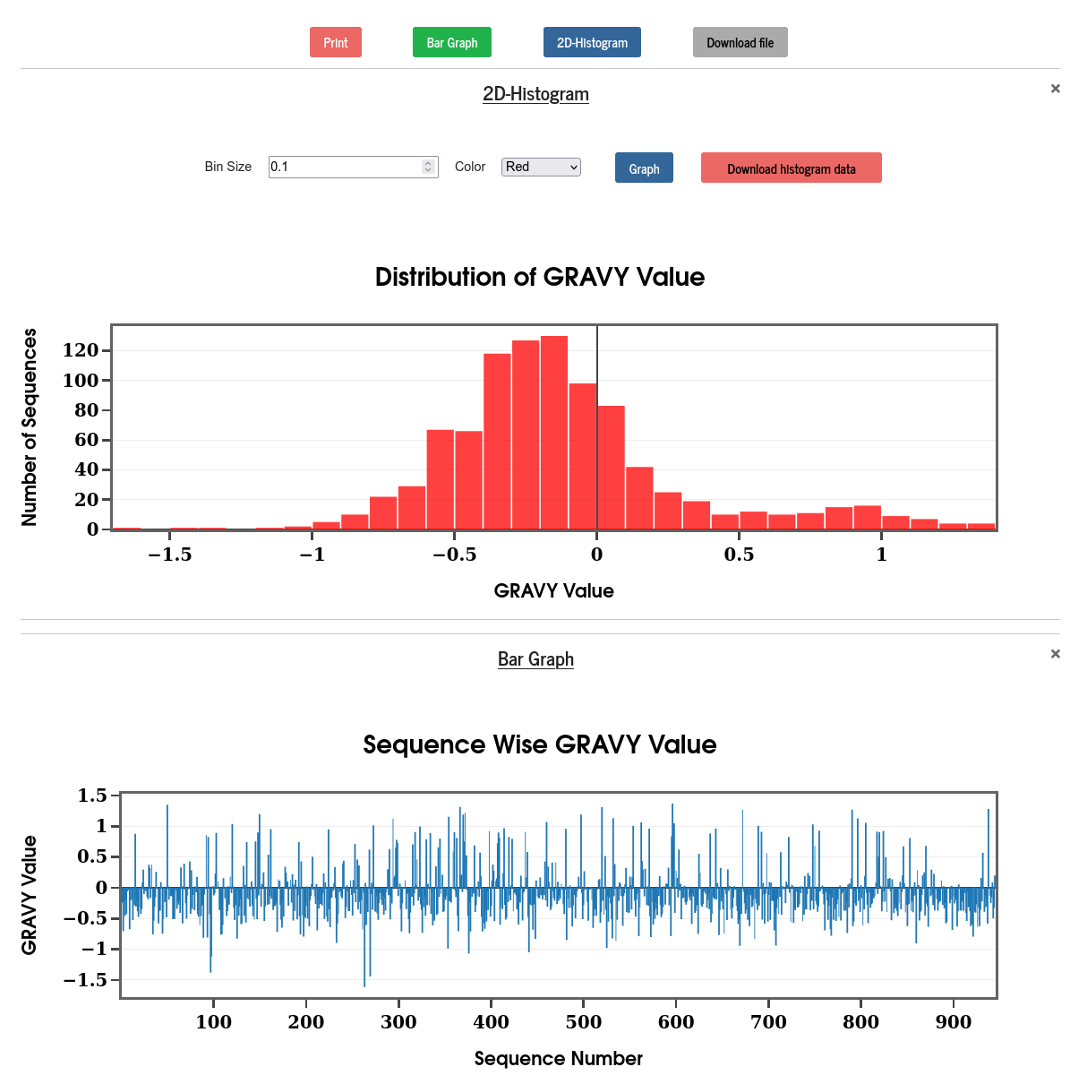
The Grand Average Hydropathy (GRAVY) value of a sequence is calculated by summing the hydropathy values of all the amino acids, divided by the total number of amino acids in the sequence. The hydropathy values are taken from Kyte & Doolittle (J. Mol. Biol. 157, 105-132 (1982)). The results are displayed in the form of a bar diagram and a 2D histogram.

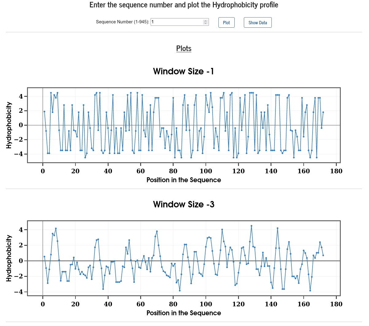
The hydrophobicity profile of a protein is calculated on all the residues using the progressive-evaluation approach with different window sizes. The window size refers to the length of the sequence used in the profile computation with the residue in question at the center of the window. The hydrophobicity score of a given residue is calculated as the sum of hydrophobicity of all the residues (Kyte & Doolittle, J. Mol. Biol. 157, 105-132 (1982)) in the window, weighted equally (100%).
The result displays hydrophobicity profile for 11 different window sizes, starting from 1 to 21 in the step of 2. One should look at the profile with window size that matches the size of the motif under investigation (Gasteiger et. al.; The Proteomics Protocols Handbook, pp.571-607, (2005)).
Users can choose the serial number of a sequence, from the top drop-down menu, to visualize the corresponding hydrophobicity profile along with the raw data in tabular format.

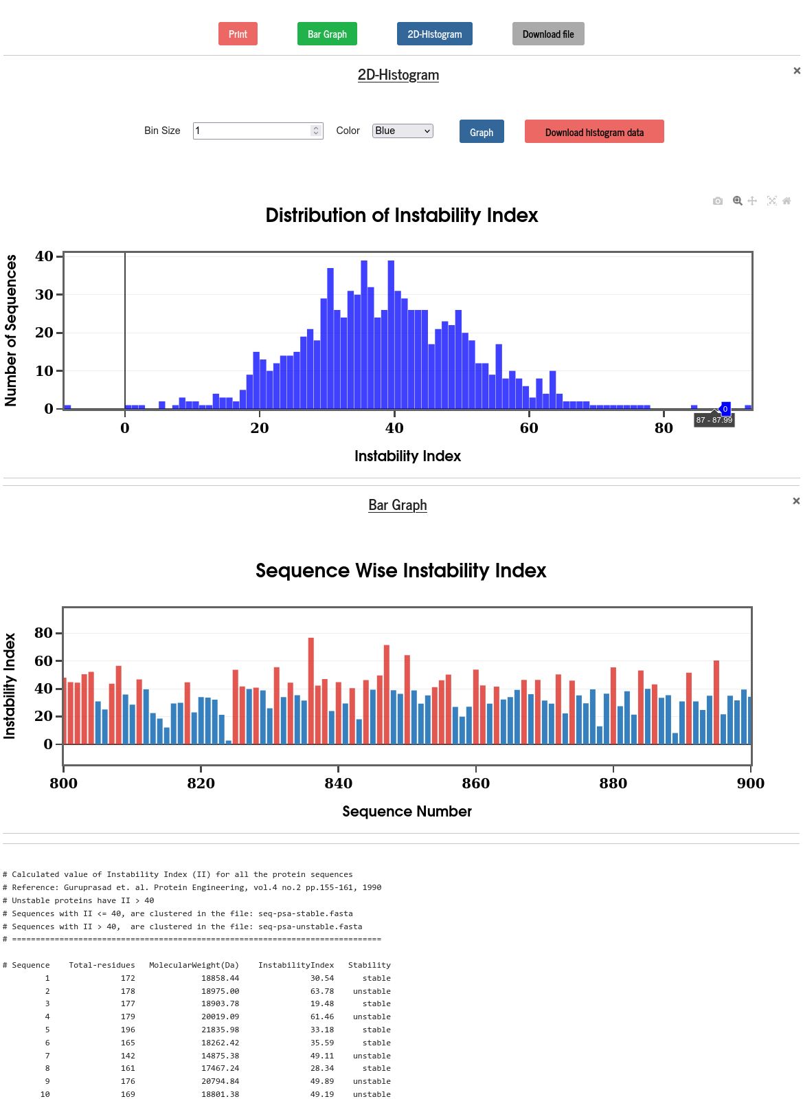
The instability index is an estimate of the stability of a protein in-vitro. Instability index (\(II\)) can be computed from the dipeptide instability weight value (\(DIWV\)) using the following scheme (Guruprasad et. al., Protein Engineering, 4(2), pp.155-161, 1990):
\(II= \frac{10}{L} \times \sum\limits_{i=1}^{L-1} DIWV(x_i,x_{i+1})\)
Where \(L\) is the length of the sequence and \(DIWV(x_i,x_{i+1})\) is the instability weight value for the dipeptide \(~x_i, x_{i+1}\) with the residues at position \(i\) and \(i+1\) in the sequence.
Protein with \(~II\) < 40 is predicted as stable and the protein is unstable if \(~II\) > 40. The results for all the sequences are displayed in the form of bar diagram and 2D-histogram. In the bar diagram, the red bars represent the unstable protein whereas the blue bars represent the stable proteins.


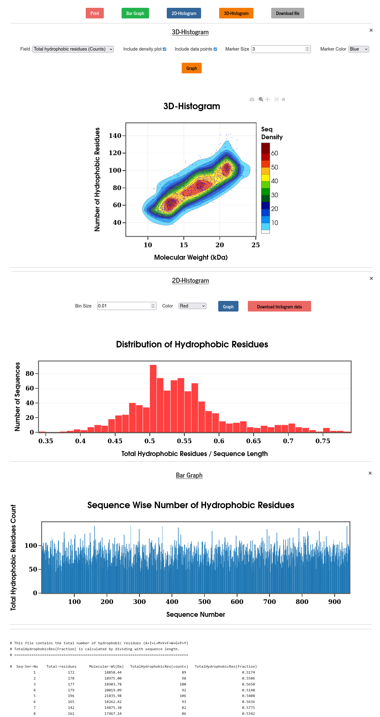
These numbers are calculated just by summing residues of respective nature-
Aliphatic residues: G, A, V, L, I, P
Aromatic residues: F, Y, W
Charged residues: K, R, D, E
Hydrophobic residues: A, I, L, M, V, F, W, G, P, Y
Polar residues: N, C, Q, S, T, H
Tiny residues: G, A, S, P
Results are displayed using bar graph, 2D & 3D distributions along with the raw data.
2. Multiple sequence alignment (MSA) data in FASTA format
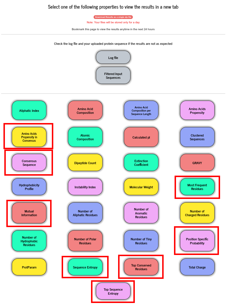
Users can upload or paste a FASTA formatted MSA file. PSA does not perform alignment of protein sequences. When this option is chosen, PSA strips off all the special characters other than the one letter amino acid codes and perform all the calculations described above, treating the MSA data as a group of sequences. From the alignment data, PSA computes a number of properties indicated with red bounding boxes and will be discussed in this section.
The sample data consists of 200 sequences of NSP6 protein of SARS-CoV-2, each 290 residues long. The sequences are mostly identical apart from a few mutations in a few sequences. Mathematically, the MSA data forms a rectangular array of alphabets representing the amino acids and “-” (1 gap):
\(A = A_i^a, ~~(i=1,...,L,~~ a=1,...,M)\)
Where \(~L~\) is the number of residues in each MSA row, and \(~M~\) is the number of MSA rows. These notations will be used below.


Position specific probability is obtained for all amino acids at every position (column) in the MSA data. This is computed from the single site reweighted frequency counts using the following formula (Morcos et al., PNAS, 108(49), E1293-E1301, 2011):
frequency of amino acid \(A\) at site \(i,~~~f_i(A) = \frac{1}{\lambda+M_{eff}} \left( \frac{\lambda}{q} + \sum\limits_{a=1}^{M} \frac{1}{m^a} \delta_{A,A_i^{a}} \right) \)
Where \(\delta_{A,B}~\) denotes the Kronecker symbol, which equals one if \(A = B\), and zero otherwise.
A single sequence is weighted by a factor \(\frac{1}{m^a}\) to correct for the sampling bias. \(~m^a\) is determined by counting the number of sequences in the MSA which are identical (pair-wise) to the sequence \(A^a\) by larger than \(xL\). The similarity threshold \(x\) can have a value in the range 0 ≤\(~x~\)≤ 1. Note that the value of \(~m^a~\) is always at least one since the sequence \(~A^a~\) is counted itself in \(~m^a~\). The total weight of all the sequences, \(~M_{eff} = \sum\limits_{a=1}^{M} 1/m^a ,~\) can be understood as the effective number of independent sequences.
In the above equation \(~q~\) is the total number of different amino acids including gap and \(~\lambda~\) is called the pseudo count. The origin of \(~\lambda~\) lies in the Bayesian statistics for calculating frequency from a sample of finite size. It also prevents counts from equalling zero and leading to divergent \(~ln(f_i(A))\).
The prescribed value of \(~x~\) is 0.8 and that of \(~\lambda~\) is 1. The default values used in PSA are: \(~\lambda = 0~\) and \(~x=1\). Using the default values of \(~\lambda~\) and \(x\), the above formula for frequency reduces to the simpler form:
\(f_i(A) = \frac{1}{M_{eff}} \sum \limits_{a=1}^{M} \frac{1}{m^a} \delta_{A, A_i^a}\)
Note that using \(~x=1~\) would reweight each sequences by the number of times it appears in the MSA, thus effectively removing the simple repeats. When the reweighting of the frequency counts is not opted, we set \(~\lambda=0~\) and \(~m^a=1~\) for all the sequences, so that \(~M_{eff}=M\). The calculated frequency or probability is printed for all sites and for all amino acids in the form of a matrix that can be viewed or downloaded as ASCII file. The most frequent amino acid at a position is the one with the highest frequency. For each position in the MSA, the most frequent residue is printed with its frequency of occurrence at that position. Residues are also arranged in decreasing order of their probability of occurrence and available under “Top Conserved Residues”.

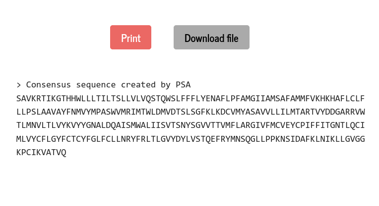
The consensus sequence is formed by putting together the most frequent residues at each position in the sequence.

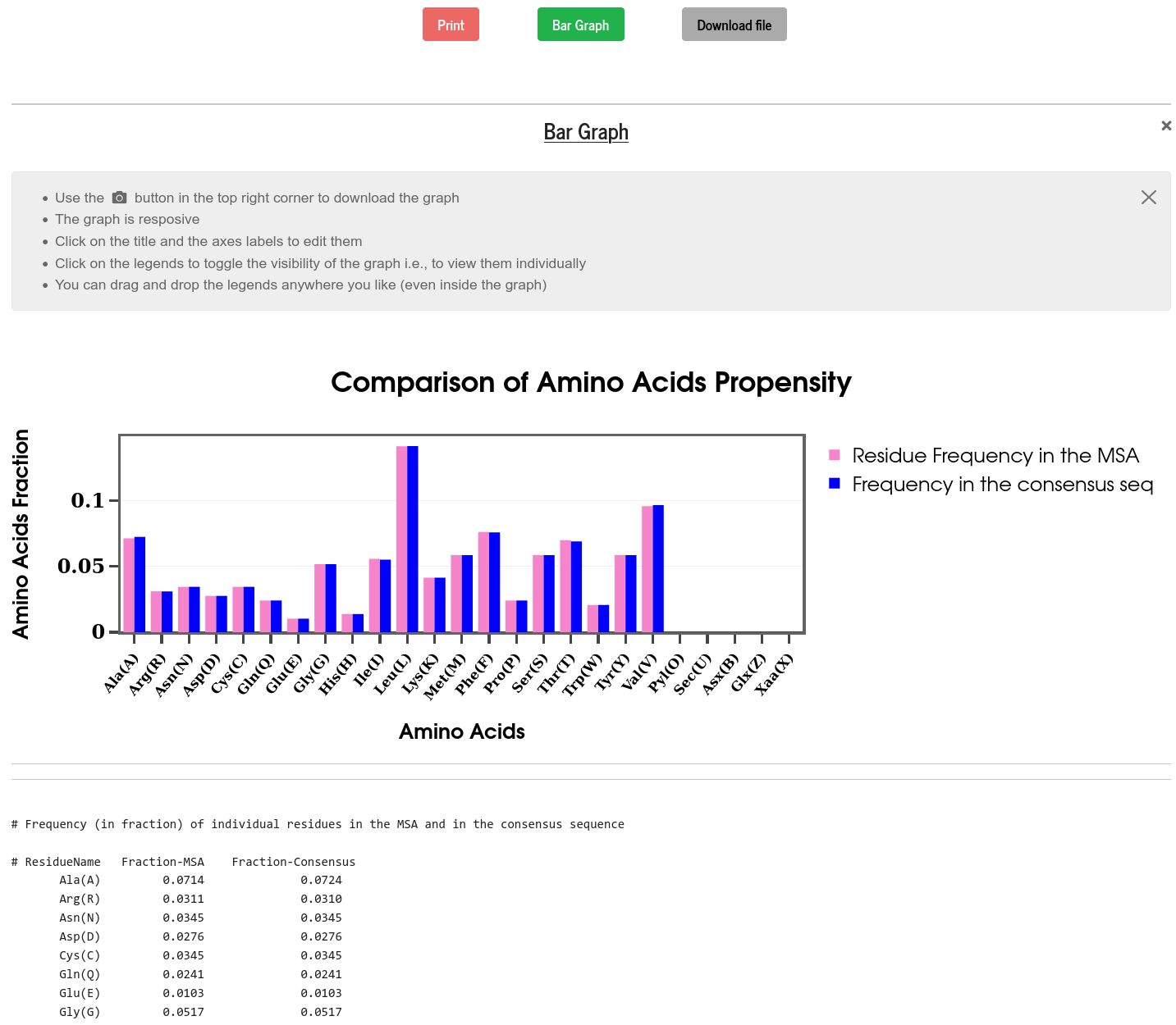
The propensity of all the amino acids is calculated from the full MSA data and from the consensus sequence and compared. To bring out the sequence biases of the consensus sequence, both the propensities are plotted, side by side, on a bar diagram. In this example, as mentioned earlier, all the sequences are almost identical and therefore show very similar propensities.


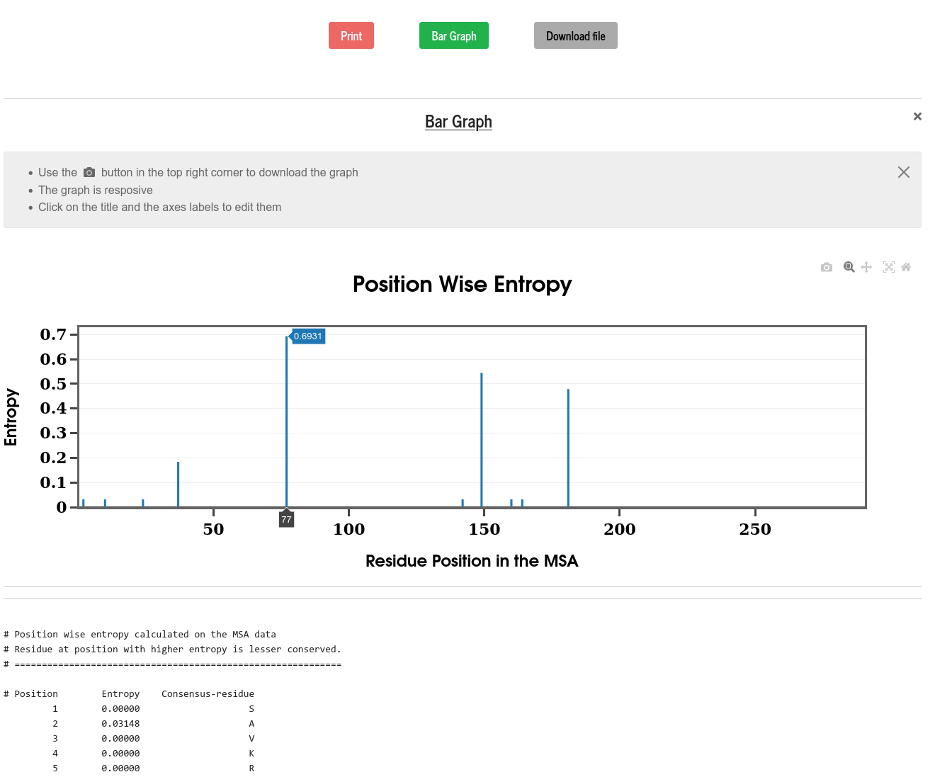
Entropy is computed for all the positions in the MSA (i.e., along the columns of MSA) using the following recipe:
\(E_i = -\sum \limits_{A} f_i(A)~~ln \left(f_i(A)\right)\)
Where \(~E_i~\) is the entropy of column \(~i~\) in the MSA. \(~f_i(A)~\) is the probability of having the amino acid \(~A~\) at column \(~i~\) in the MSA and the summation is over all the \(q\) amino acids.
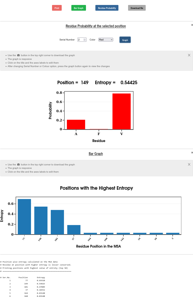
PSA calculates the position-wise entropy and displays it in the form of a bar diagram. The positions in the sequence with “Entropy spike” are those with the most mutations. The top 50 entropy values with the positions are also printed and can be visualized in a bar graph. One can also select the serial number from the top entropy list to check the mutations and fraction of occurrence of different amino acids at that position in the sequence.

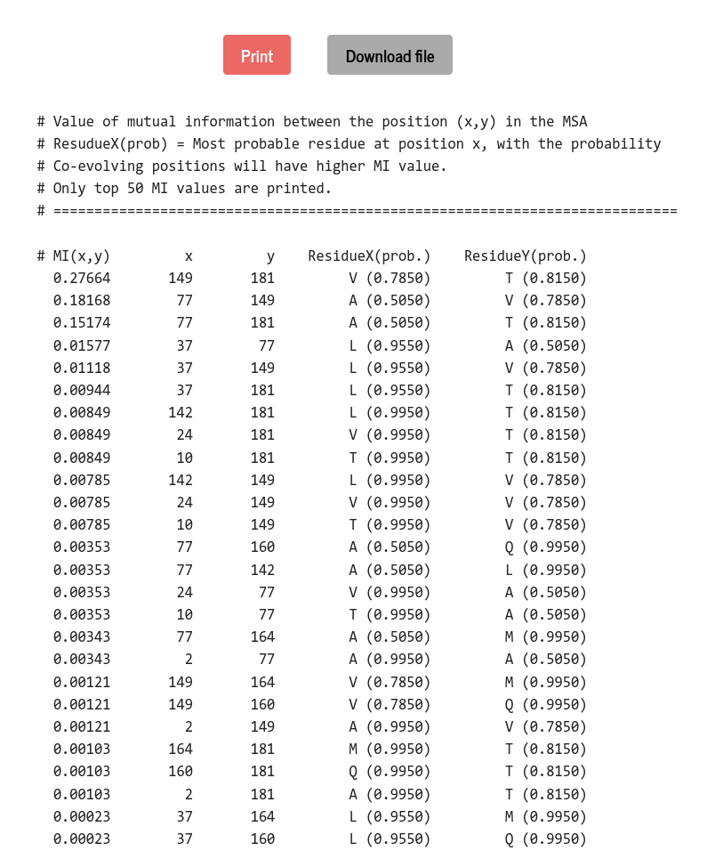
Mutual information (MI) is a measure of correlated changes at a pair of positions in the MSA data. MI is defined in terms of the joint and the marginal probabilities as :
\(MI_{ij} = \sum \limits_{A,B} f_{ij}(A,B)~ln\left( \frac{f_{ij}(A,B)}{f_i(A)~f_j(B)} \right) \)
Where the joint probability of finding residue \(~A~\) and \(~B~\) at position \(~i~\) and \(~j~\) is, \(f_{ij}(A,B) = \frac{1}{\lambda + M_{eff}} \left( \frac{\lambda}{q^2} + \sum \limits_{a=1}^{M} \frac{1}{m^a}~\delta_{A,A_i^a}~\delta_{B,A_j^a}\right) \). If the columns \(~i~\) and \(~j~\) are statistically independent, the joint distribution would factorize into \(f_i(A) \times f_j(B)\) and \(MI_{ij} = 0\). \(~MI_{ij}>0\) when the columns \(~i~\) and \(~j~\) are statistically correlated. Correlation is higher for larger values of \(MI_{ij}\).
PSA prints a maximum of 50 \(MI_{ij}\) values for a pair of positions \(~i~\) and \(~j~\) along with the most frequent residues at those positions.
Website Tested On
| OS | Version | Chrome | Firefox | Microsoft Edge | Safari |
|---|---|---|---|---|---|
| Linux | Ubuntu 20.04 | 96.0.4664.110 | 95.0 | n/a | n/a |
| MacOS | Monterey | 96.0.4664.110 | 86.0.1 | n/a | 15.1 |
| Windows | 10 | 96.0.4664.110 | 95.0.1 | 96.0.1054.62 | n/a |